Mean Reversion Strategy Research: SPY Dip-Buying Analysis
Introduction
"Buy the dip" is one of the most common retail trading strategies. The premise is simple: when prices fall sharply, they tend to revert to the mean, creating a buying opportunity. This research tests whether a systematic dip-buying strategy can outperform passive buy-and-hold investing on SPY (S&P 500 ETF) while maintaining a high win rate.
SPY returned 247% from 2015-2024, including the COVID crash of 2020 and the bear market of 2022. This serves as the benchmark to beat.
Objective
This study attempts to build a rules-based "buy the dip" strategy that meets the following criteria:
- Win rate > 65% on dip-buying trades
- Profit factor > 1.5 (average win > average loss)
- Total return > 247% (beating SPY buy-and-hold over 2015-2024)
- Maximum 30 trades per year
- Consistent performance in both bull markets (2017, 2019, 2021) and bear markets (2022)
Methodology
A backtesting framework was built to analyze 10 years of SPY data (2015-2024). Over 40 strategy variations were implemented and tested.
Phase 1: Dip Signal Analysis
The first step was to analyze forward returns after various "dip" conditions.
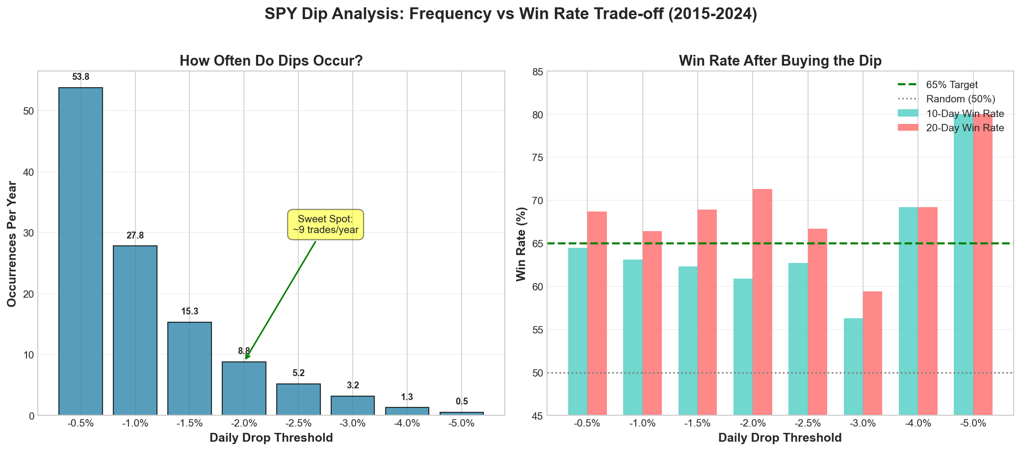
Figure 1: Frequency vs. win rate trade-off across different dip thresholds.
Single-day drops of 2%+:
- Frequency: ~9 times per year
- 10-day forward win rate: 61%
- 20-day forward win rate: 71%
RSI < 25 (deeply oversold):
- Frequency: ~6 times per year
- 5-day forward win rate: 80%
Drawdown > 10% from 20-day high:
- Frequency: ~6-7 times per year
- 10-day forward win rate: 75%
- 20-day forward win rate: 80%
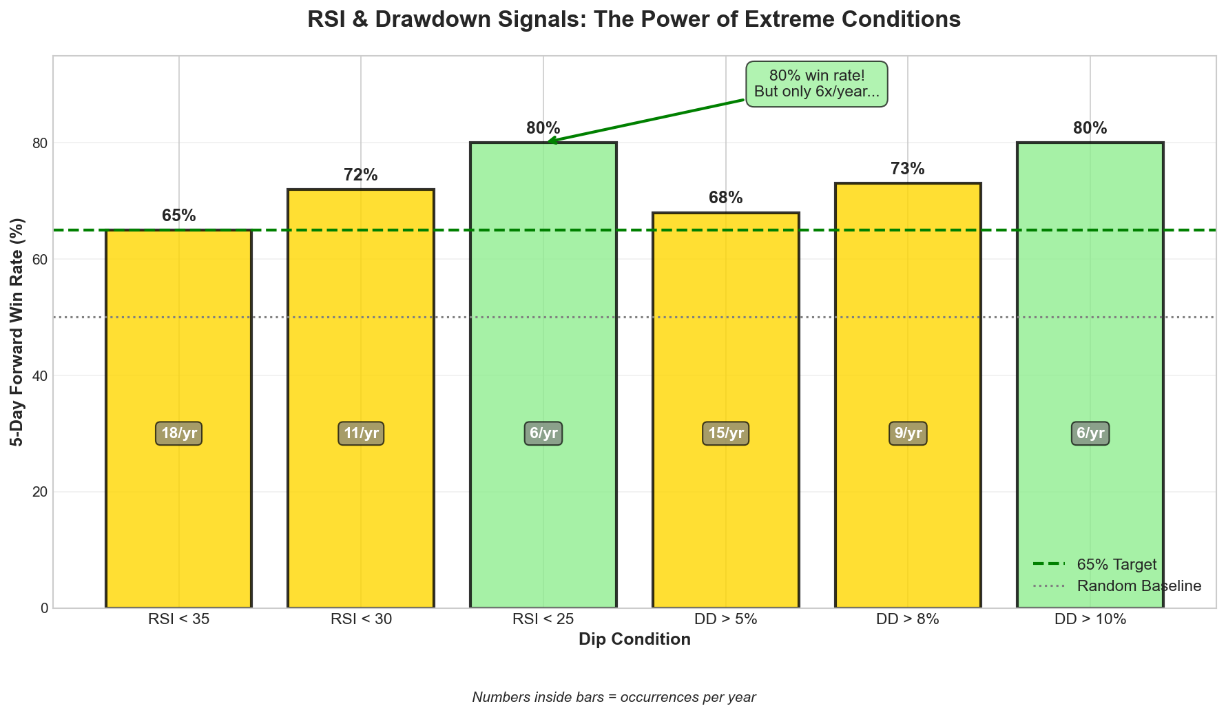
Figure 2: RSI and drawdown conditions show high win rates but low frequency.
Phase 2: The Return Problem
Initial strategies based on high-conviction dips produced:
- 80%+ win rate
- Profit factor > 2.0
- Only 5-6 trades per year
- Total return: 48%
The 48% return over 10 years significantly underperformed buy-and-hold (247%). The ultra-selective approach resulted in only ~5% time invested, missing the bull market gains.
Dip-detection implementation:
def detect_dip_signals(data: pd.DataFrame, rsi_threshold: int = 30,
                       drawdown_threshold: float = 0.08) -> pd.DataFrame:
    """
    Generate buy signals when extreme oversold conditions are met.
    """
    signals = data.copy()

    # Calculate RSI (14-period)
    delta = signals['Close'].diff()
    gain = delta.where(delta > 0, 0).rolling(window=14).mean()
    loss = (-delta.where(delta < 0, 0)).rolling(window=14).mean()
    rs = gain / loss
    signals['RSI'] = 100 - (100 / (1 + rs))

    # Calculate drawdown from 20-day high
    signals['rolling_high'] = signals['Close'].rolling(window=20).max()
    signals['drawdown'] = (signals['Close'] - signals['rolling_high']) / signals['rolling_high']

    # Generate signals
    signals['signal'] = 0
    signals.loc[signals['RSI'] < rsi_threshold, 'signal'] = 1
    signals.loc[signals['drawdown'] < -drawdown_threshold, 'signal'] = 1

    return signals
Finding: High win rate does not correlate with high total returns when time-in-market is low.
Phase 3: Trend-Following Hybrid
To increase time-in-market, strategies were redesigned:
- Stay invested during uptrends (above 200-day MA)
- Use dips as entry signals
- Exit only on confirmed trend breaks (death cross: 50 MA < 200 MA)
def trend_following_with_dip_entry(data: pd.DataFrame) -> pd.DataFrame:
    """
    Hybrid approach: trend-following with dip-timed entries.
    Entry: Buy on dip (RSI < 35) when above 200 MA
    Exit: Death cross (50 MA crosses below 200 MA)
    """
    signals = data.copy()

    signals['MA_50'] = signals['Close'].rolling(window=50).mean()
    signals['MA_200'] = signals['Close'].rolling(window=200).mean()

    delta = signals['Close'].diff()
    gain = delta.where(delta > 0, 0).rolling(window=14).mean()
    loss = (-delta.where(delta < 0, 0)).rolling(window=14).mean()
    signals['RSI'] = 100 - (100 / (1 + gain / loss))

    signals['uptrend'] = signals['MA_50'] > signals['MA_200']
    signals['entry'] = (signals['RSI'] < 35) & signals['uptrend']
    signals['exit'] = signals['MA_50'] < signals['MA_200']

    return signals
Results:
- Return: 237%
- Win rate: 100% (5 trades)
- Profit factor: Infinite
The 237% return still underperformed buy-and-hold (247%). The death cross exit in early 2022 avoided the drawdown but also missed the subsequent recovery.
Phase 4: Multi-Signal Exit
More aggressive exit conditions were tested using multiple bearish indicators:
- Price below 50-day MA
- Negative 20-day momentum (< -5%)
- MACD bearish crossover
- RSI < 45
Exit triggered when 3+ conditions were met.
def multi_signal_exit(data: pd.DataFrame) -> pd.DataFrame:
    """Exit when multiple bearish signals align."""
    signals = data.copy()

    signals['MA_50'] = signals['Close'].rolling(50).mean()
    signals['momentum_20d'] = signals['Close'].pct_change(20) * 100

    exp12 = signals['Close'].ewm(span=12).mean()
    exp26 = signals['Close'].ewm(span=26).mean()
    signals['MACD'] = exp12 - exp26
    signals['MACD_signal'] = signals['MACD'].ewm(span=9).mean()

    delta = signals['Close'].diff()
    gain = delta.where(delta > 0, 0).rolling(14).mean()
    loss = (-delta.where(delta < 0, 0)).rolling(14).mean()
    signals['RSI'] = 100 - (100 / (1 + gain / loss))

    signals['bearish_count'] = (
        (signals['Close'] < signals['MA_50']).astype(int) +
        (signals['momentum_20d'] < -5).astype(int) +
        (signals['MACD'] < signals['MACD_signal']).astype(int) +
        (signals['RSI'] < 45).astype(int)
    )

    signals['exit'] = signals['bearish_count'] >= 3
    return signals
Results ("tactical no-early" strategy):
- Return: 317% (beats buy-and-hold)
- Profit factor: 7.18
- Trades/year: 2.8
- Average win: 18.1%
- Average loss: -1.5%
- Win rate: 43%
This strategy beat buy-and-hold but failed the 65% win rate criterion. The high return came from asymmetric payoffs (18.1% avg win vs 1.5% avg loss), not from win rate.
Phase 5: The Trade-off Triangle
Analysis revealed a fundamental constraint in dip-buying strategies:
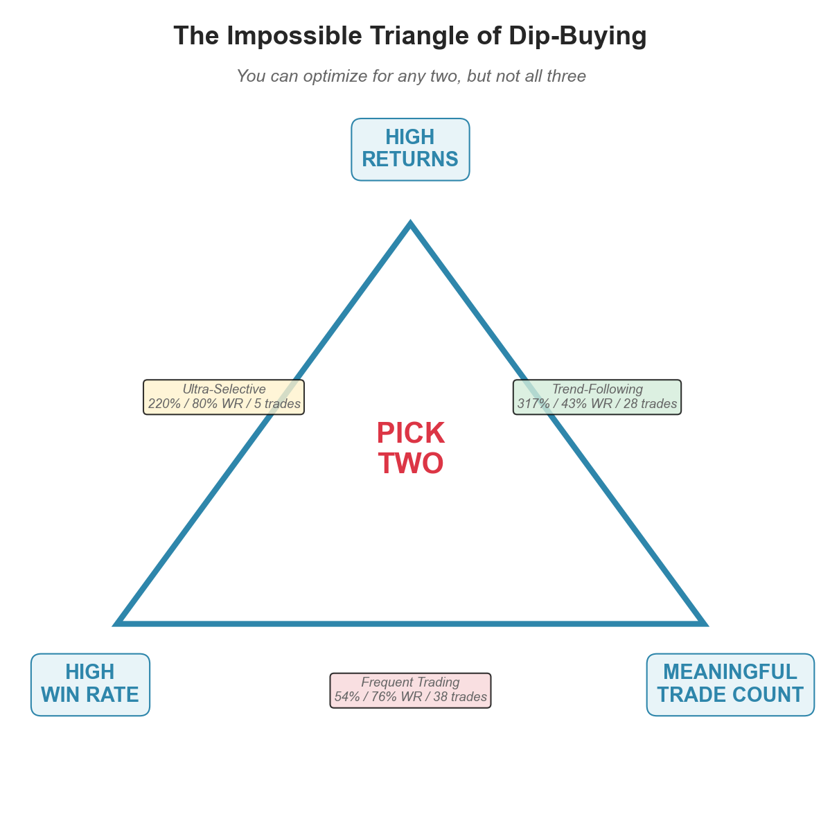
Figure 3: Three-way trade-off between returns, win rate, and trade frequency.
The three criteria form mutually exclusive pairs:
- High returns + High win rate = Very few trades (statistically insignificant)
- High returns + Meaningful trades = Low win rate (trend-following characteristics)
- High win rate + Meaningful trades = Low returns (insufficient time-in-market)
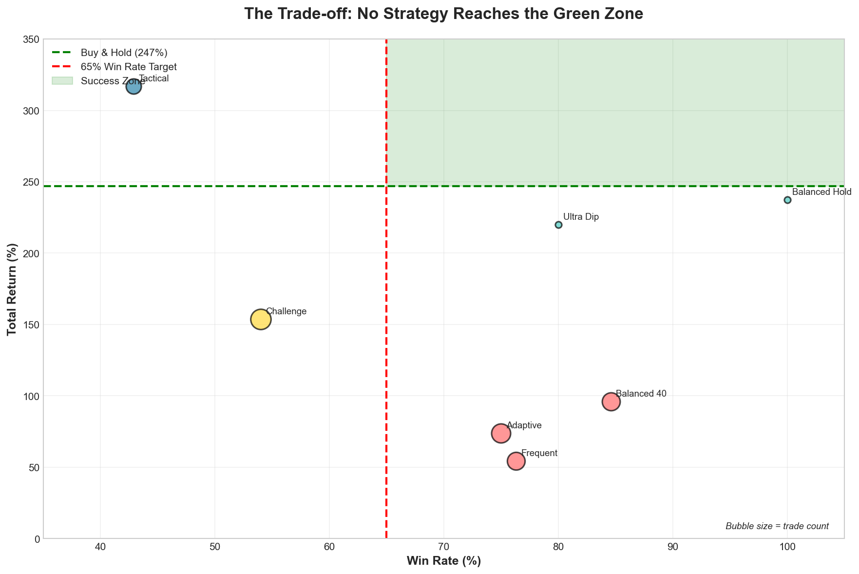
Figure 4: All tested strategies fall outside the target zone (>247% return AND >65% win rate).
The 2022 Bear Market
The 2022 bear market provided a stress test for dip-buying strategies:
- SPY annual return: -18.6%
- Number of -2% daily drops: 23
- Win rate on buying those dips: 48%
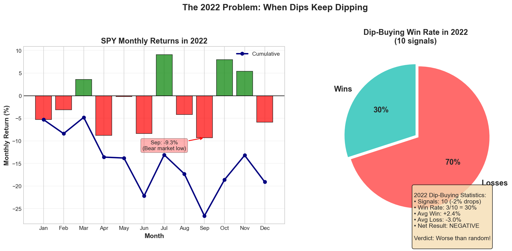
Figure 5: Dip-buying performance during the 2022 bear market.
Dip-buying assumes mean reversion to an upward trend. In a bear market, the trend is downward, causing mean reversion strategies to underperform.
Strategies that exited on trend breaks avoided the 2022 drawdown but missed the 2023-2024 recovery. Strategies that remained invested captured the recovery but experienced the full drawdown.
Key Findings
1. Mean Reversion as Entry Timing
Mean reversion signals (RSI oversold, drawdowns) are effective for entry timing but insufficient as a complete strategy due to low time-in-market.
2. Win Rate vs. Returns
Win rate and total returns showed no positive correlation in this study. The highest-returning strategy (317%) had only 43% win rate. The relationship between win rate and profitability depends on the reward-to-risk ratio:
def calculate_expectancy(win_rate: float, avg_win: float, avg_loss: float) -> float:
    """
    Calculate expected return per trade.
    Example: 40% win rate with 6:1 ratio = 0.4 * 6 + 0.6 * (-1) = +1.8
    Example: 90% win rate with 1:10 ratio = 0.9 * 1 + 0.1 * (-10) = -0.1
    """
    return (win_rate * avg_win) + ((1 - win_rate) * avg_loss)
3. Selectivity Trade-off
Ultra-selective signals (RSI < 25) produced 80% win rates but only 6 trades per year, resulting in insufficient market exposure for competitive returns.
4. Bear Market Performance
All dip-buying strategies tested showed degraded performance during the 2022 bear market. Mean reversion assumptions break down when the underlying trend reverses.
Results Summary
| Strategy | Return | Win Rate | Beats B&H? | Meets 65% WR? | Trades/Yr |
|---|---|---|---|---|---|
| Tactical No-Early | 317% | 43% | Yes | No | 2.8 |
| Balanced Hold | 237% | 100% | No | Yes | 0.5 |
| Ultra Dip | 220% | 80% | No | Yes | 0.5 |
| Frequent Trading | 54% | 76% | No | Yes | 3.8 |
No strategy achieved all target criteria simultaneously.
Conclusion
The challenge criteria (>247% return, >65% win rate, meaningful trade frequency) appear to be mutually exclusive for simple rules-based strategies on SPY.
The fundamental trade-off between time-in-market (required for returns) and selectivity (required for win rate) creates a constraint that prevents simultaneous optimization of both metrics.
Experiments: 40+ Strategies tested: 14 core strategies with parameter variations Time period: 2015-2024 Asset: SPY
Appendix: Backtesting Framework
from dataclasses import dataclass
from typing import List, Dict
import pandas as pd
import numpy as np

@dataclass
class BacktestResult:
    """Results from a backtest run."""
    total_return: float
    annual_return: float
    max_drawdown: float
    sharpe_ratio: float
    win_rate: float
    profit_factor: float
    num_trades: int
    trades: List[Dict]

class Backtester:
    """Backtesting engine for long-only strategies."""

    def __init__(self, initial_capital: float = 10000, commission: float = 0.001):
        self.initial_capital = initial_capital
        self.commission = commission

    def run(self, data: pd.DataFrame, signals: pd.DataFrame) -> BacktestResult:
        """Execute backtest and return performance metrics."""
        cash = self.initial_capital
        shares = 0
        position = 0
        trades = []
        portfolio_values = []
        entry_price = 0
        entry_date = None

        for date, row in signals.iterrows():
            close = row['Close']
            signal = row.get('signal', 0)

            if signal == 1 and position == 0:
                shares = (cash * (1 - self.commission)) / close
                cash = 0
                position = 1
                entry_price = close
                entry_date = date

            elif signal == -1 and position == 1:
                proceeds = shares * close * (1 - self.commission)
                cash = proceeds
                pnl_pct = (close - entry_price) / entry_price * 100
                trades.append({
                    'entry_date': entry_date,
                    'exit_date': date,
                    'entry_price': entry_price,
                    'exit_price': close,
                    'pnl_pct': pnl_pct
                })
                shares = 0
                position = 0

            portfolio_values.append(cash + shares * close)

        portfolio = np.array(portfolio_values)
        total_return = (portfolio[-1] - self.initial_capital) / self.initial_capital * 100

        wins = [t for t in trades if t['pnl_pct'] > 0]
        losses = [t for t in trades if t['pnl_pct'] <= 0]

        win_rate = len(wins) / len(trades) * 100 if trades else 0
        avg_win = np.mean([t['pnl_pct'] for t in wins]) if wins else 0
        avg_loss = abs(np.mean([t['pnl_pct'] for t in losses])) if losses else 0.01
        profit_factor = avg_win / avg_loss if avg_loss > 0 else 999

        return BacktestResult(
            total_return=total_return,
            annual_return=total_return / 10,
            max_drawdown=self._calculate_max_drawdown(portfolio),
            sharpe_ratio=self._calculate_sharpe(portfolio),
            win_rate=win_rate,
            profit_factor=profit_factor,
            num_trades=len(trades),
            trades=trades
        )

    def _calculate_max_drawdown(self, portfolio: np.ndarray) -> float:
        peak = np.maximum.accumulate(portfolio)
        drawdown = (portfolio - peak) / peak * 100
        return abs(drawdown.min())

    def _calculate_sharpe(self, portfolio: np.ndarray, rf: float = 0.02) -> float:
        returns = np.diff(portfolio) / portfolio[:-1]
        excess = returns - rf / 252
        return np.sqrt(252) * excess.mean() / excess.std() if excess.std() > 0 else 0